Scientific Python at Microscopy & MicroAnalysis 2019
Today, I presented a talk titled “Scientific Python: A Mature Computational Ecosystem for Microscopy” [PDF] at the Microscopy and MicroAnalysis conference in Portland.
A few members of the audience familiar with scientific Python told me they had learned something, so I’ll highlight the few topics that I think may have qualified.
SciPy 1.0 paper #
The first official release of SciPy was in 2001, and a mere 16 years later we reached 1.0. This says a lot about the developer community, and how careful they are to label their own work as “mature”! To celebrate this project milestone, we published a preprint on arXiv that outlines the project history and its current status. It mentions, among other achievements, that SciPy was instrumental in the first gravitational wave detection, as well as the recent imaging of the black hole in Messier 87.
NumPy __array_function__ protocol
#
The 1.17 release of NumPy (2019-07-26) has support for a new array function protocol, that allows external libraries to pass their array-like objects through NumPy without them being horribly mangled. E.g., you may call NumPy’s sum on a CuPy array: the computation will happen on the GPU, and the resulting array will still be a CuPy array.
Here is an example:
In [24]: import cupy as cp

In [25]: x = cp.random.random([10, 10])

In [26]: y = x.sum(axis=0)

In [27]: type(y), y.shape
Out[27]: (cupy.core.core.ndarray, (10,))

In [28]: import numpy as np

In [29]: z = np.sum(x, axis=0)

In [30]: type(z), z.shape
Out[30]: (cupy.core.core.ndarray, (10,))
Note how the result is the same, whether you use CuPy or NumPy’s sum.
Whereas NumPy used to be the reference implementation for array computation in Python, it is fast evolving into a standard API, implemented by multiple libraries.
PyTorch and TensorFlow easily consume Python images #
Images in scientific Python (scikit-image, opencv, etc.) are represented as NumPy arrays. It is trivial to pass these arrays into deep learning libraries such as TensorFlow:
from tensorflow.keras.applications.inception_v3 import (
    InceptionV3, preprocess_input, decode_predictions
)
from skimage import transform

net = InceptionV3()

def inception_predict(image):
    # Rescale image to 299x299, as required by InceptionV3
    image_prep = transform.resize(image, (299, 299, 3), mode='reflect')

    # Scale image values to [-1, 1], as required by InceptionV3
    image_prep = (img_as_float(image_prep) - 0.5) * 2

    predictions = decode_predictions(
        net.predict(image_prep[None, ...])
    )

    plt.imshow(image, cmap='gray')

    for pred in predictions[0]:
        (n, klass, prob) = pred
        print(f'{klass:>15} ({prob:.3f})')
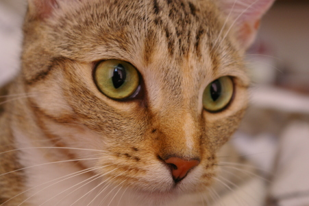
Chelsea the Cat
For example, when running inception_predict on skimage.data.chelsea(), I get:
Egyptian_cat (0.904)
       tabby (0.054)
   tiger_cat (0.035)
        lynx (0.000)
 plastic_bag (0.000)
Looks about right!
imglyb #
Philipp Hanslovsky, at SciPy2019, demonstrated his Python ↔ Java bridge called imglyb. In contrast to many previous efforts, this library allows you to share memory between Python and Java, avoiding costly (and, potentially fatal, dependent on memory constraints) reallocations. E.g., he showed how to manipulate volumes of data (3-D arrays) in Python, and to then view those using ImageJ’s impressive BigDataViewer, which can rapidly slice through the volume at an arbitrary plane.
Lazy viewing of data using dask
#
This is a trick I borrowed from Matt Rocklin’s blog post.
When you have a number of large images that, together, form a stack (3-D volume), it may not be possible to load the entire stack into memory. Instead, you can use dask to lazily access parts of the volume on an as-needed basis.
This is achieved in four steps:
-
Convert
skimage.io.imreadinto a delayed function, i.e. instead of returning the image itself it returns adaskDelayedobject (similar to a Future or a Promise), that can fetch the image when needed. -
Use this function to load all images. The operation is instantaneous, returning a list of
Delayedobjects. -
Convert each
Delayedobject to adaskArray. -
Stack all of these
daskArrays to form the volume.
Note that each one of these steps should execute almost instantaneously; no images files are accessed on disk: that only happens once we start operating on the dask Array volume.
Here is the code:
from glob import glob

from dask import delayed
import dask.array as da

from skimage import io

# Read one image to get dimensions
image = io.imread('samples/Test_TIRR_0_1p5_B0p2_01000.tiff')

# Turn imread into a delayed function, so that it does not immediately
# load an image file from disk
imread = delayed(io.imread, pure=True)

# Create a list of all our samples; since a delayed version of `imread`
# is used, no work is done immediately
samples = [imread(f) for f in sorted(glob('samples/*.tiff'))]

# Convert each "delayed" object in the list above into a dask array
sample_arrays = [da.from_delayed(sample, shape=image.shape, dtype=np.uint8) for sample in samples]

# Stack all these arrays into a volume
vol = da.stack(sample_arrays)
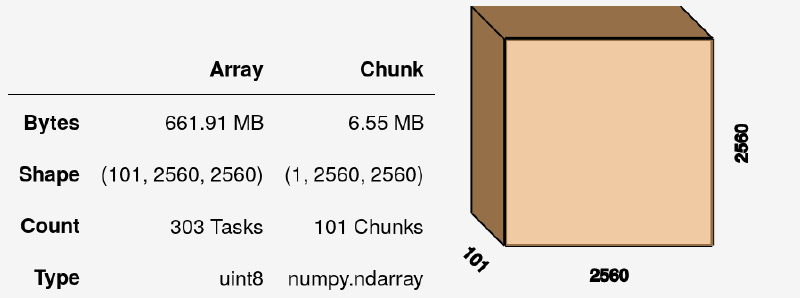
I have 101 slices of 2048x2048 each, so the resulting dask Array volume (at this stage fully virtual, without any data inside) is:
We can do numerous operations on this array, such as summing it with vol.sum(axis=0), although this still yields an uncomputed dask Array. To get actual values, we need to call:
vol.sum(axis=0).compute()
Napari #
To visualize a volume like the one above, I could have sliced into it and displayed the result using matplotlib. However, I used this opportunity to play around with a brand new open source image viewer called Napari.
Napari allows you to visualize layers interactively, similarly to GIMP or Photoshop. In Napari’s case, these layers can be images, labels, points, and a few others.
While this isn’t explicitly documented (Napari is still in alpha!), I had some insider knowledge (👋 J!) that Napari supports both dask and Zarr arrays. So, we can pass in our volume from the example above as follows:
import napari

with napari.gui_qt():
    viewer = napari.view(vol, clim_range=(0, 255))
(Instead of the context manager, you may also use %gui = qt in Jupyter or IPython.)
I also happened to have ground truth labels available, so I loaded those up the same way I did the volume, and added it to the visualization:
viewer.add_labels(labels, name='Labels')
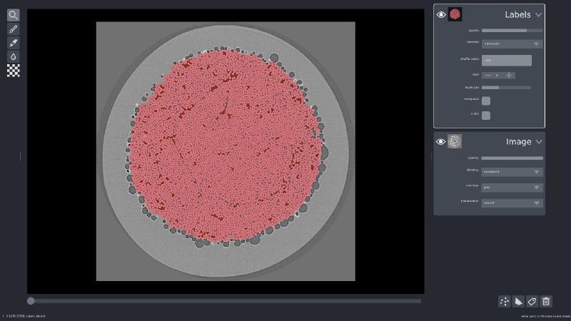
If you’d like to play with Napari yourself, I have a 3D cell segmentation example available online.
Community #
Toward the conclusion of my talk, I emphasized the role of community in building healthy scientific software ecosystems. In the end, it is all about people. I briefly highlight two community groups:
-
PanGeo, whom I think sets a great example of how to organize field-specific interest around existing open source tools, and building scalable online analysis platforms without reinventing the wheel.
-
OME, the Open Microscopy Environment, who is leading the charge on open data exchange formats for microscopy. Interestingly, it looks like Zarr—the chunked, compressed array container—may well be part of the next open standard they recommend.
Conclusion #
Thank you to the organizers of M&M 2019 for inviting me to speak; I very much enjoyed our session, and look forward to working with this community on making scientific Python an even better platform for mirocroscopy analysis!